Clustering of EU countries
Oct 27, 2018 00:00 · 1320 words · 7 minute read
In this article I used a public Eurostat dataset, to develop a segmentation of the EU countries. This dataset consists of 5 confidence indicators:
- Consumer Confidence Indicator
- Construction confidence indicator
- Industrial confidence indicator
- Retail confidence indicator
- Services Confidence Indicator
These indicators are formed via qualitative surveys which are conducted on a monthly basis in the following areas: manufacturing industry, construction, consumers, retail trade, services and financial services. These surveys started in 1980 and gradually include all the new EU members. About 137,000 firms and more than 41,000 consumers are currently surveyed every month across the EU.
The used metrics is the balance i.e. the difference between positive and negative answers (in percentage points of total answers), as index, as confidence indicators (arithmetic average of balances).
More information about these surveys can be found at this link
The eurozone consists of 19 countries: Austria, Belgium, Cyprus, Estonia, Finland, France, Germany, Greece, Ireland, Italy, Latvia, Lithuania, Luxembourg, Malta, the Netherlands, Portugal, Slovakia, Slovenia, and Spain.
The Eurostat package used to obtain the original datasets.
More details about the ETL steps can be found, in the actual code, at the link at the end of the article.
ETL & Exploratory Analysis
The original dataset consists of 11,340 observations that include these indicators for EU countries on a monthly basis. In the processed dataset I used i) observations from 2014 onward & ii) the median values of each variable for each state, so finally the dataset consists of 28 observations in total. One more variable was created, by averaging all Business related confidence indicators (Construction, Industrial, Retail & Services Confidence Indicators), to use a general business confidence indicator.
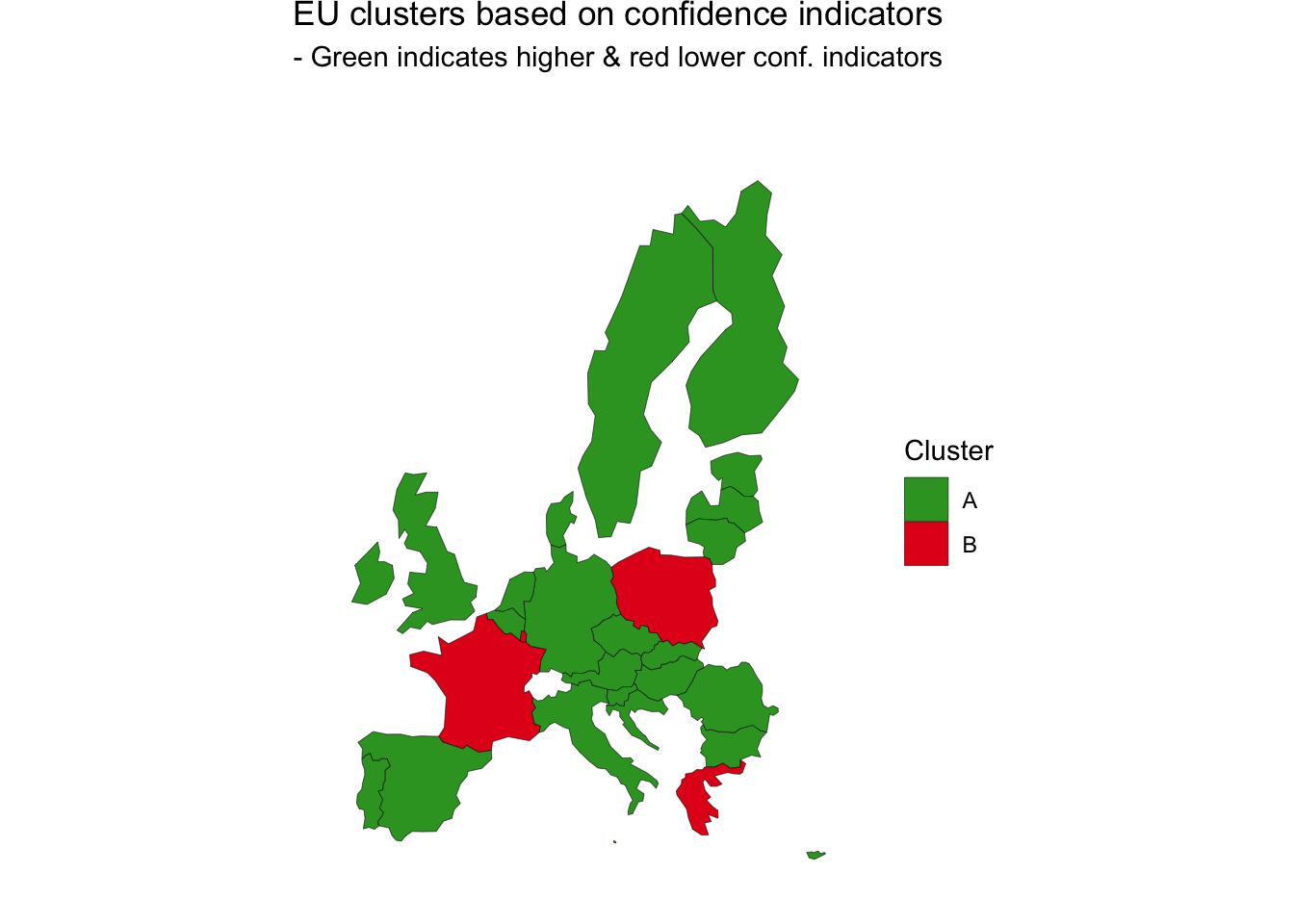
It would be interesting to see the map plots of the confidence indicators. Below there are plots with the consumer & averaging business confidence indicators.
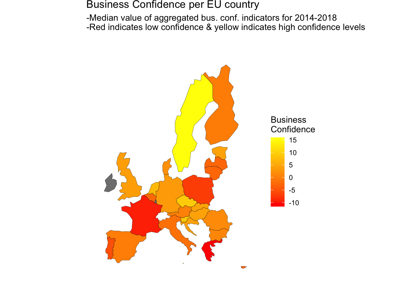
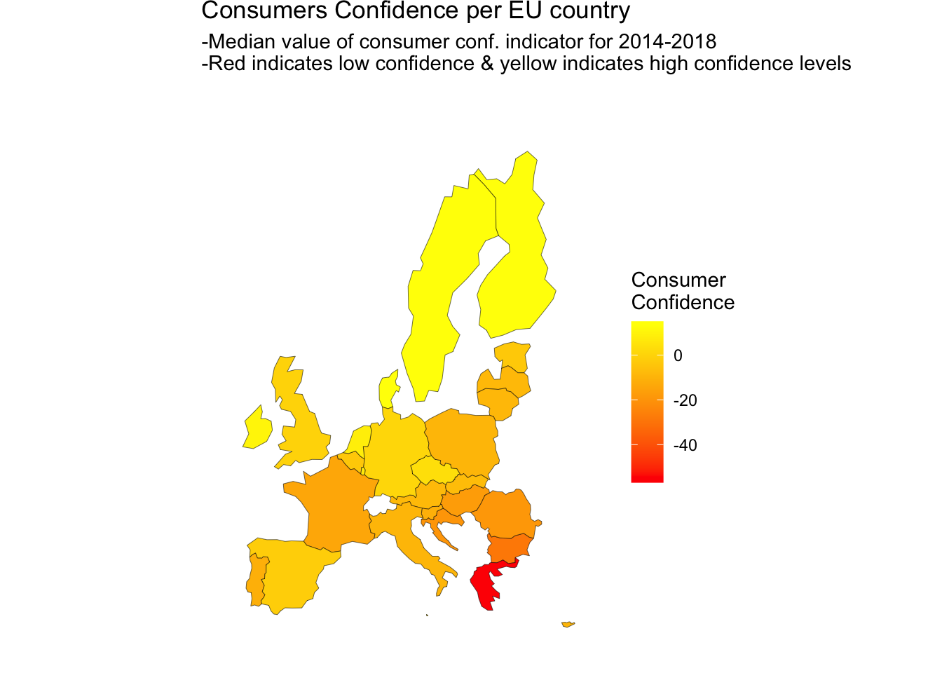
- It is clear that there are significant differences between countries.
- Northern Europe countries tend to have higher consumers confidence
indicators.
- There are some outliers here. E.g. Greece has significantly lower confidence indicator than the rest of the nations.
Below there is a scatterplot with marker labels indicating the positioning of each country in respect to consumer and business confidence indicators.
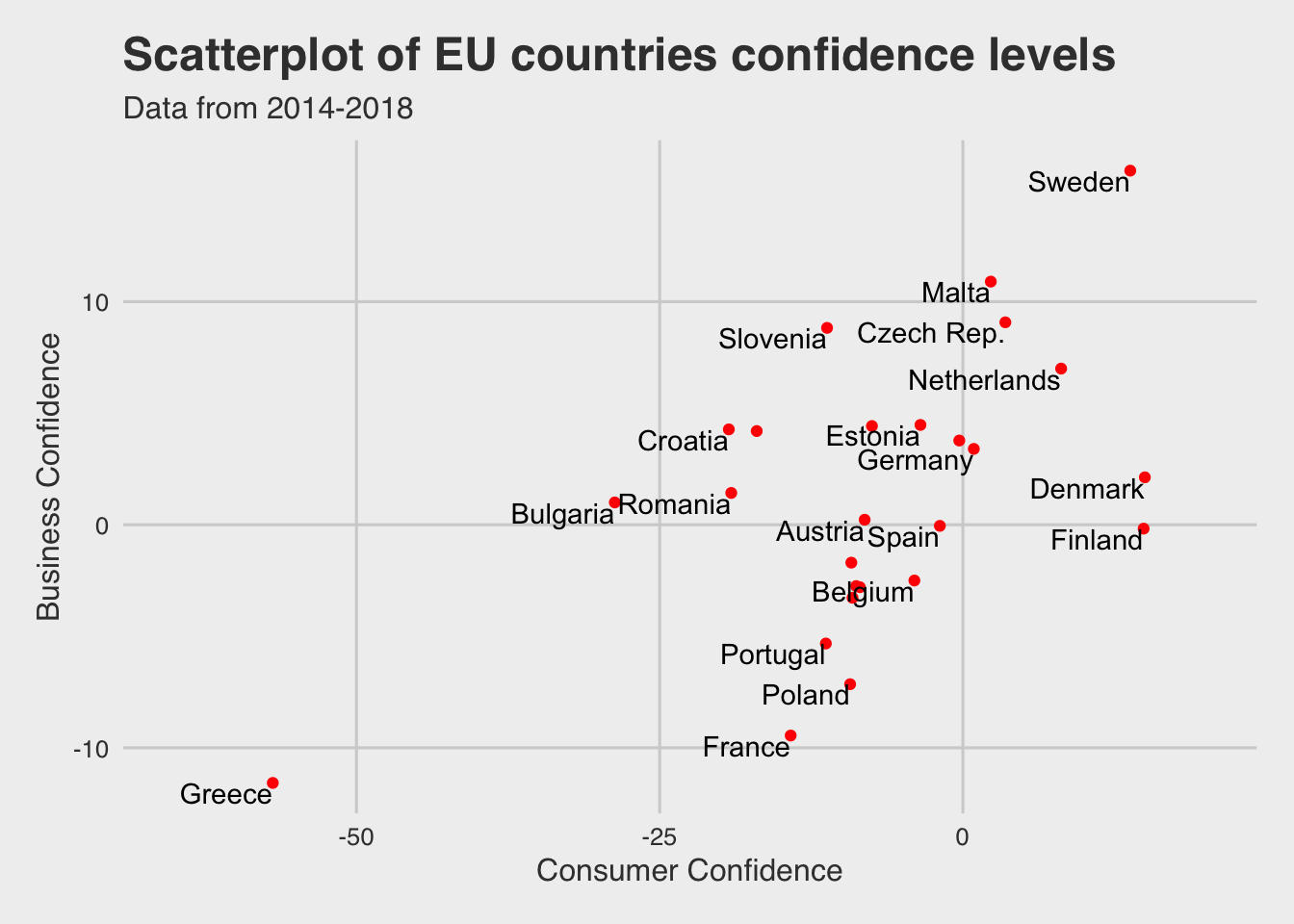
We can indicate some patterns from the plot above, similar to the findings before:
- There are some outliers, such as Greece(bottom left) & Sweden(top right)
- There is a group of countries that are placed in the middle of the plot, indicating
average consumer & business confidence
- In all countries, the business confidence is substantially higher than
consumer confidence
Segmentation
Since there are quite a few differences between countries regarding
confidence indicators, it would be interesting to develop a segmentation, to check how well the countries are forming teams.
The k-means algorithm used for the segmentation.
It is the widest used unsupervised learning algorithm. The procedure follows
a simple and easy way to classify a given data set through a certain number of
clusters (assume k clusters) fixed apriori. The main idea is to define k centers,
one for each cluster. These centers should be placed in a cunning way because of
different location causes different result. So, the better choice is to place
them as much as possible far away from each other. The next step is to take each
point belonging to a given data set and associate it to the nearest center. When
no point is pending, the first step is completed and an early group age is done.
At this point we need to re-calculate k new centroids as barycenter of the clusters
resulting from the previous step. After we have these k new centroids, a new
binding has to be done between the same data set points and the nearest new center.
A loop has been generated. As a result of this loop we may notice that the k
centers change their location step by step until no more changes are done or in
other words centers do not move any more.
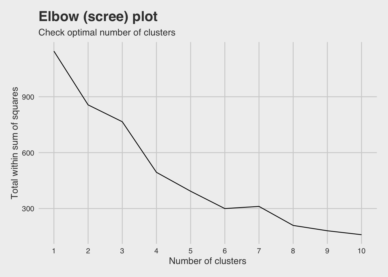
Indicate suitable number of clusters
The elbow (scree) plot below, is used to check for the suitable number of clusters. So what we are looking for, is the point at which the curve in the plot begins to flatten out.
In detail, the total within cluster sum of squares is calculated (the sum of euclidean distances between each observation and the centroid corresponding to the cluster to which the observation is assigned).
Silhouette analysis
In general, silhouette analysis determines how well each of the observations fit into corresponding cluster (Higher values are better).
It involves calculating a measurement called the silhouette width for every
observation:
- A value close to 1 suggests that this observation is well matched to its current cluster.
- A value of 0 suggests that it is on the border between two clusters and possibly
belong to either one.
- A value close to -1 indicates that the observation has a better fit to its
closest neighbouring cluster.
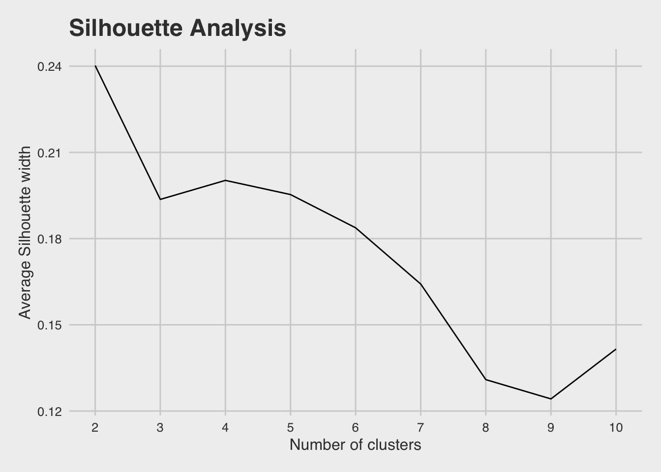
In conclusion, I proceed with 2 clusters, as it is more suitable both from a technical & practical point of view.
Below there is a table plot with information about all clusters, indicating the mean value of each confidence indicator within the cluster
| cluster | n | Construction | Consumer | Industrial | Retail | Services |
|---|---|---|---|---|---|---|
| A | 24 | -10.44 | -4.10 | 0.62 | 7.02 | 13.67 |
| B | 4 | -22.85 | -18.42 | -9.00 | -1.30 | 1.23 |
Cluster A tend to have higher values than cluster B on Construction confidence indicator, Consumer confidence indicator & Services Confidence Indicator
Both clusters tend to have similar values on Industrial confidence indicator & Retail confidence indicator
Principal components
It would be nice to plot these clustering results and check these out visually.
But it is impossible to visualise so many variables, as various dimensions are
required.
One way to overcome this is to use some dimensionality reduction technique. In particular, PCA (principal components analysis) is used.
It finds structure in features and aid in visualization.
In particular:
- It will find some linear combination of variables to create principal components (new features)
- Maintain most variance in the data
- Principal components (new features) are uncorrelated (i.e. orthogonal to each other)
The plot below (bi-plot) shows all the original observations plotted on the first two principal components.
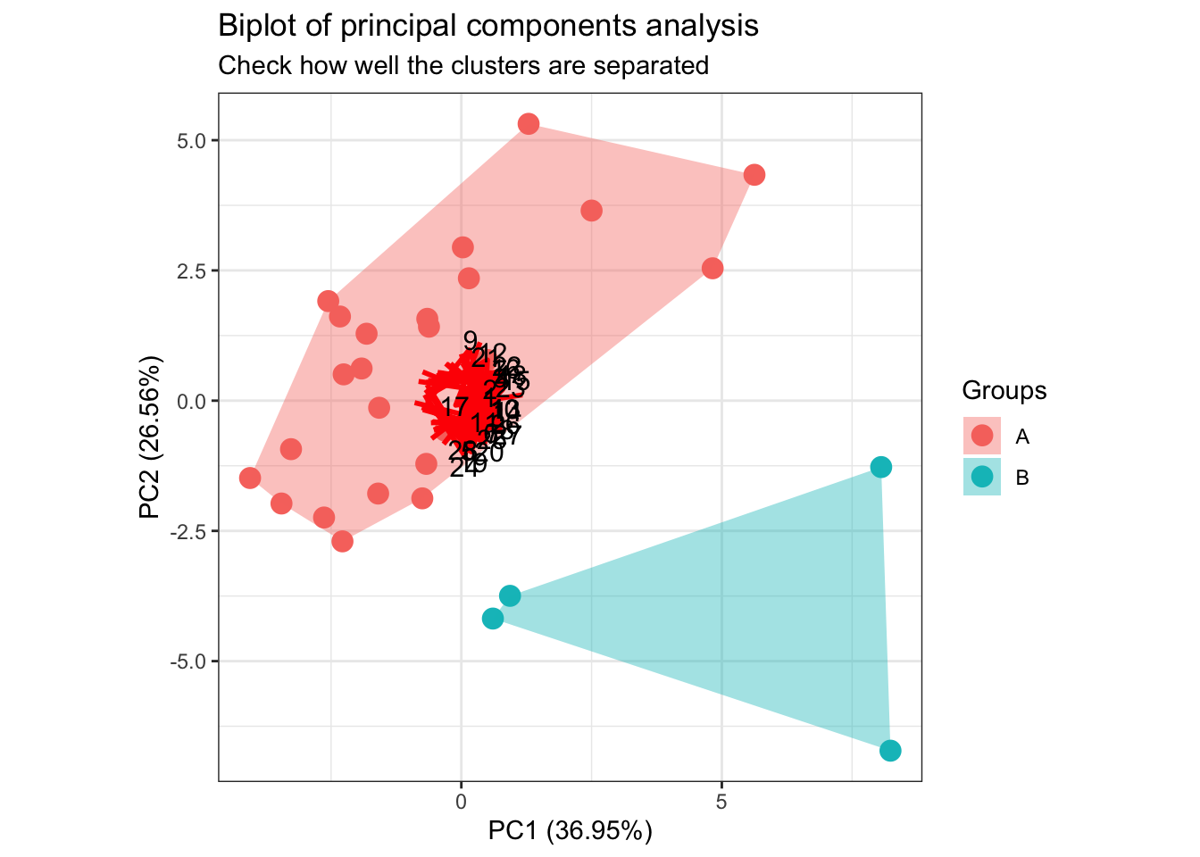
- The A cluster clearly stands out from cluster B
- There is just a minor overlap
- In general, northern Europe countries tend to have higher confidence indicators that place them in cluster A
- The clustering results can confirm the theory of the two-speed EU (significant differences between countries in many aspects as the standard of living etc.)
Below there is a table of all EU countries indicating their cluster and the median confidence indicators (since 2014)
| Country | Cluster | Construction | Consumer | Industrial | Retail | Services |
|---|---|---|---|---|---|---|
| Austria | A | -3.7 | -8.1 | -3.5 | -7.1 | 15.2 |
| Belgium | A | -13.9 | -4.0 | -4.3 | -7.0 | 15.2 |
| Bulgaria | A | -21.7 | -28.7 | 0.6 | 15.3 | 9.8 |
| Cyprus | A | -28.4 | -9.1 | -1.8 | -0.9 | 18.0 |
| Czech Rep. | A | -19.7 | 3.5 | 3.1 | 19.8 | 33.1 |
| Germany | A | -2.2 | 0.9 | 1.0 | -3.7 | 18.5 |
| Denmark | A | -4.3 | 15.0 | -3.9 | 8.5 | 8.2 |
| Estonia | A | -3.0 | -3.5 | 2.6 | 12.5 | 5.8 |
| Spain | A | -28.4 | -1.9 | -1.6 | 11.3 | 18.5 |
| Finland | A | -4.0 | 14.9 | -3.0 | -4.7 | 11.0 |
| Croatia | A | -11.2 | -19.3 | 4.4 | 8.0 | 15.9 |
| Hungary | A | -5.1 | -17.0 | 5.7 | 9.1 | 7.1 |
| Italy | A | -19.8 | -9.2 | -1.3 | 6.4 | 7.9 |
| Lithuania | A | -19.7 | -8.8 | -6.4 | 5.5 | 9.6 |
| Latvia | A | -19.3 | -8.5 | -2.7 | 6.1 | 4.7 |
| Malta | A | 4.4 | 2.3 | 4.7 | 6.1 | 28.4 |
| Netherlands | A | 10.7 | 8.1 | 1.6 | 6.9 | 8.8 |
| Portugal | A | -31.8 | -11.3 | -0.5 | 1.3 | 9.7 |
| Romania | A | -13.3 | -19.1 | 0.4 | 10.5 | 8.1 |
| Sweden | A | 15.7 | 13.8 | 3.7 | 17.7 | 26.4 |
| Slovenia | A | -7.0 | -11.2 | 6.3 | 16.7 | 19.3 |
| Slovakia | A | -10.0 | -7.5 | 4.7 | 15.7 | 7.3 |
| United Kingdom | A | -4.5 | -0.3 | 4.4 | 7.4 | 7.8 |
| Ireland | A | NA | 10.6 | NA | NA | NA |
| Greece | B | -45.2 | -56.9 | -6.3 | 2.1 | 3.1 |
| France | B | -29.2 | -14.2 | -3.4 | -4.4 | -0.8 |
| Luxembourg | B | 5.2 | 6.7 | -15.7 | -5.7 | NA |
| Poland | B | -22.2 | -9.3 | -10.6 | 2.8 | 1.4 |