Exploratory Analysis

During exploratory analysis, we try to discover patterns in the time series such as:
- Trend A pattern involving long-term increase or decrease in the time series
- Seasonality A period pattern exists due to the calendar (e.g. quarter, month, weekday)
- Cyclicity A pattern exists where the data exhibits rise and fall that are not of a fixed period (duration usually of at least two years)

Below there is a time series plot of the Eurozone countries quarterly GDP since 1995.

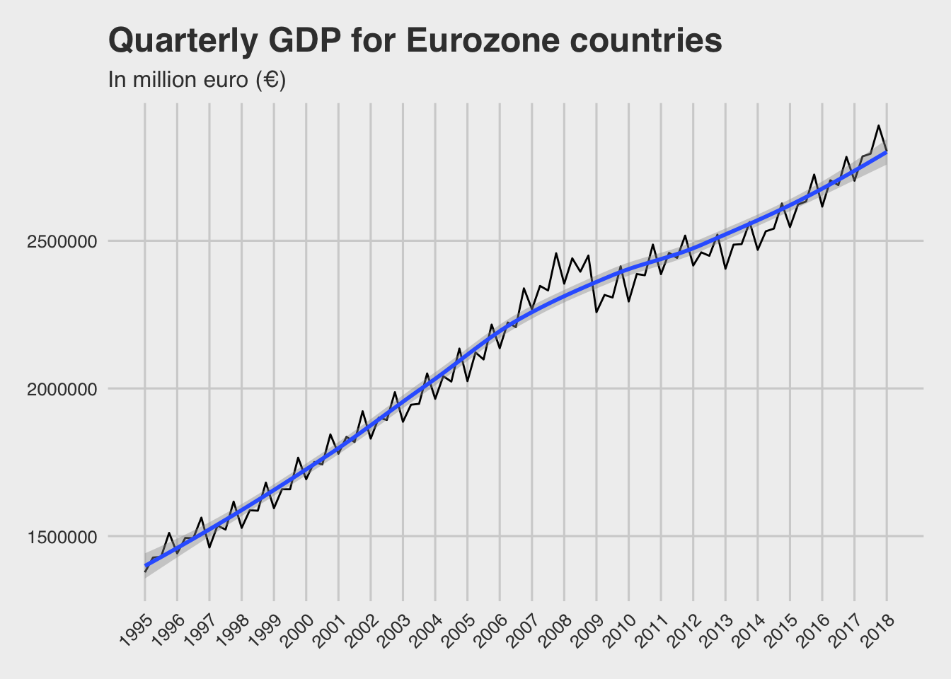
There are a few outputs from the time series plot above:
- We can say that there is an overall positive trend
- There is no noticeable increased/decreased variability in the trend
- It looks that there is some seasonality, but needs further investigation
- There is no cyclicity
- There is a significant disruption in GDP growth around years 2008-9

A seasonal plot is used below to investigate seasonality. A seasonal plot is similar to a time plot except that the data are plotted against the individual “seasons” in which the data were observed.

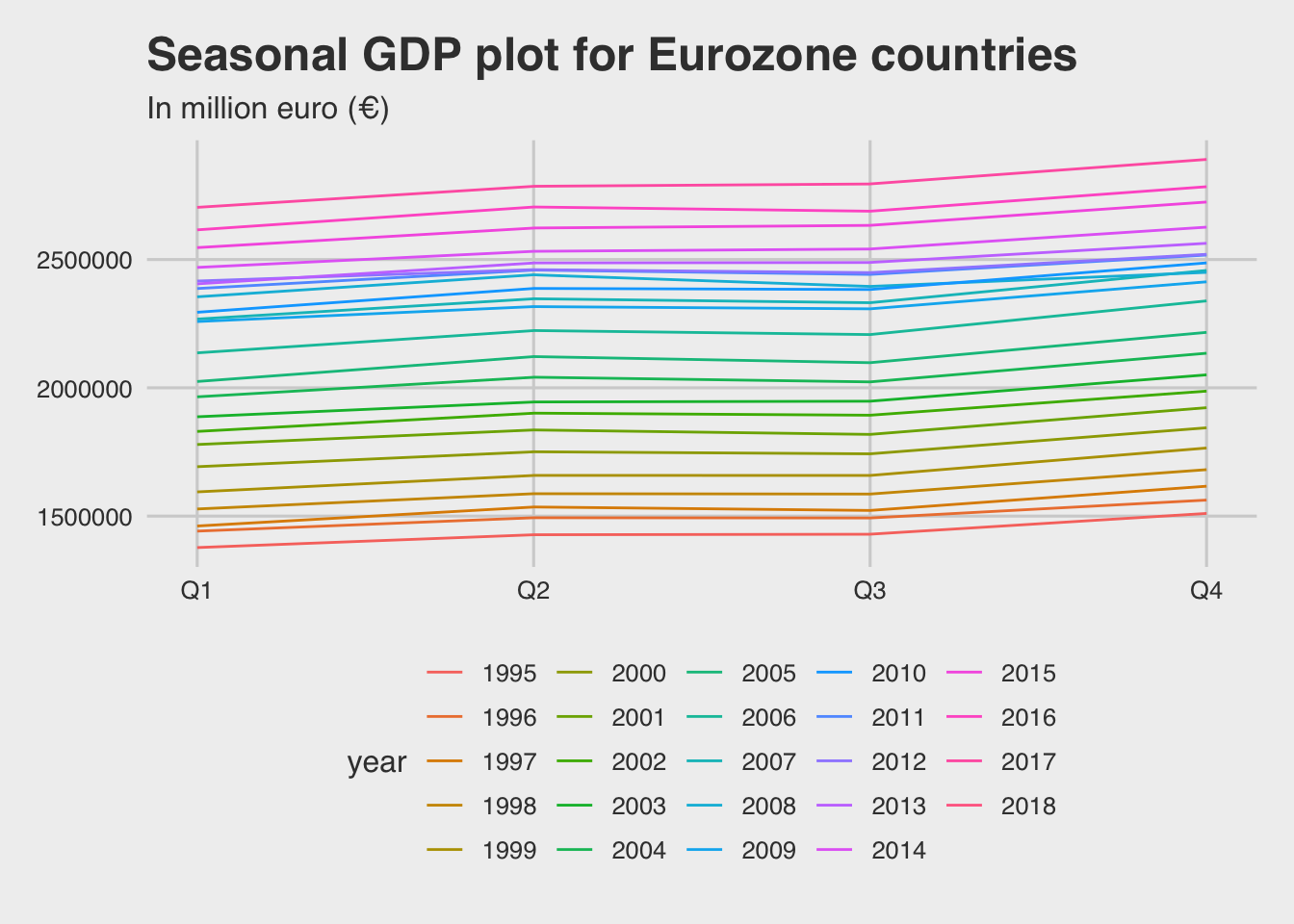
This strengthens our confidence for seasonality in the time series. It seems that the 4th quarter is always the higher, while the 1st is the lowest in each year. The 2nd & 3rd are about the same.

A lag plot will help us understand if there is autocorrelation in the time series. Another way to look at time series data is to plot each observation against another observation that occurred some time previously. For example, you could plot yt against yt−1. This is called a lag plot because you are plotting the time series against lags of itself. Basically it is a scatterplot between the time series and the lagged values of the time series.

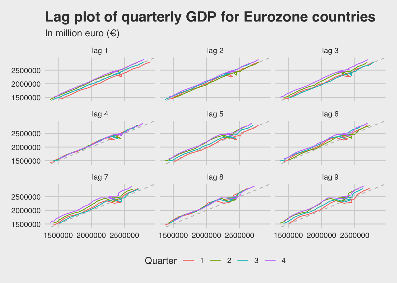
There is a strong seasonality at lag 4 (1 year), as all quarters line plots follow an almost identical path.

Below there is an autocorrelation function plot. The correlations associated with the lag plots form what is called the autocorrelation function (ACF). Spices that exceeds the confidence intervals (blue lines) indicates that autocorrelation with specific lag is statistically significant (different than zero)

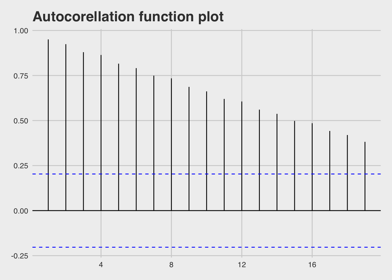
It looks that there are significant autocorrelations at all lags, which indicates a trend and/or seasonality in the time series.

We can also use the Ljung-Box test to test if the time series is white noise. White noise is a time series that is purely random. Below there is a test at lag 4.

## 
##  Box-Ljung test
## 
## data:  gdp_ts
## X-squared = 319.62, df = 4, p-value < 2.2e-16

Ljung-Box test p-value is very small < 0.01, so there is strong evidence that the time series is not white noise and has seasonality and/or trend.

Modelling

ARIMA (Auto-regressive integrated moving average) models provide one of the main approaches to time series forecasting. It is the most widely-used approach to time series forecasting, and aim to describe the autocorrelations in the data.

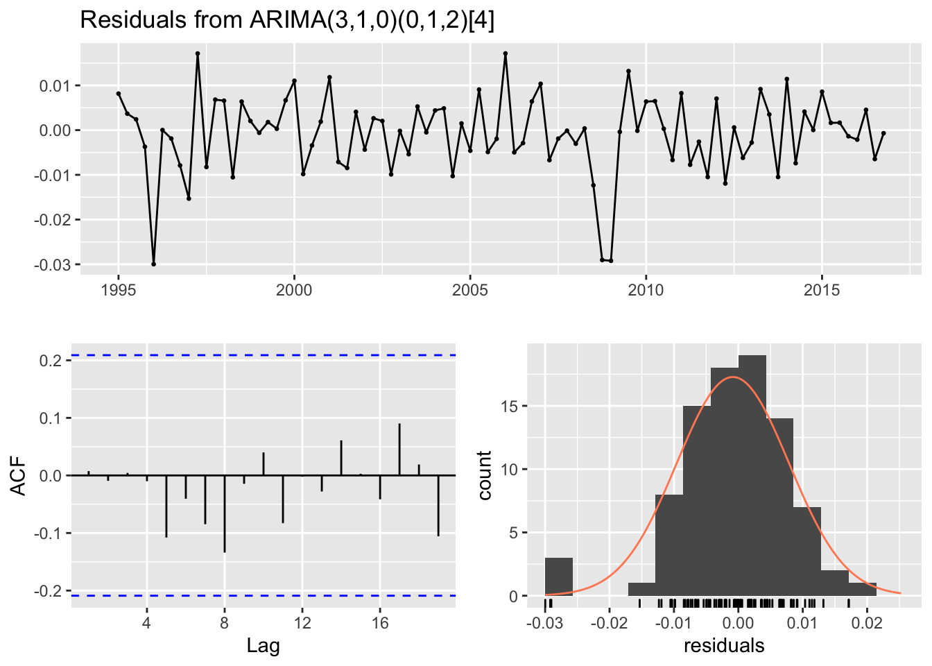
The final fitted model was produced by the auto.arima() function of the forecast library. It rapidly estimates a series of model and return the best, according to either AIC, AICc or BIC value. After fitting the ARIMA model, it is essential to check that the residuals are well-behaved (i.e., no outlines or patterns) and resemble white noise. Below there are some residual plots for the fitted ARIMA model.

## 
##  Ljung-Box test
## 
## data:  Residuals from ARIMA(3,1,0)(0,1,2)[4]
## Q* = 3.7729, df = 3, p-value = 0.2871
## 
## Model df: 5.   Total lags used: 8

We can say that the model is fairly good, since the residuals are closely normally distributed, have no real pattern and autocorrelations are not significant.
The final model is a seasonal ARIMA(2,1,1)(0,1,1)[4]. Both seasonal and first differences have been used, indicated by the middle slot in each part of the model. Also, one lagged error and one seasonally lagged error has been selected, indicated by the last slot in each part of the model. Two autoregression terms have been used, indicated by the first slot in the model. No seasonal autoregression terms have been used.

Finally, the accuracy of the forecasting model is examined. Below there is a test for the model accuracy, using all four quarters in 2017 & the 1st quarter of 2018 as a test set.

##                     ME     RMSE      MAE         MPE     MAPE      MASE
## Training set -1939.741 18227.96 13162.32 -0.08904229 0.636205 0.1914578
## Test set     53381.557 55964.14 53381.56  1.90697066 1.906971 0.7764830
##                    ACF1 Theil's U
## Training set 0.05467523        NA
## Test set     0.05995906 0.7616938

MAPE (Mean absolute percentage error) for the test set is 1.68, so we can conclude that the prediction accuracy of the model is around 98.3 %.

Below there is a time series plot of the Eurozone countries quarterly GDP forecasts for 2018-19.

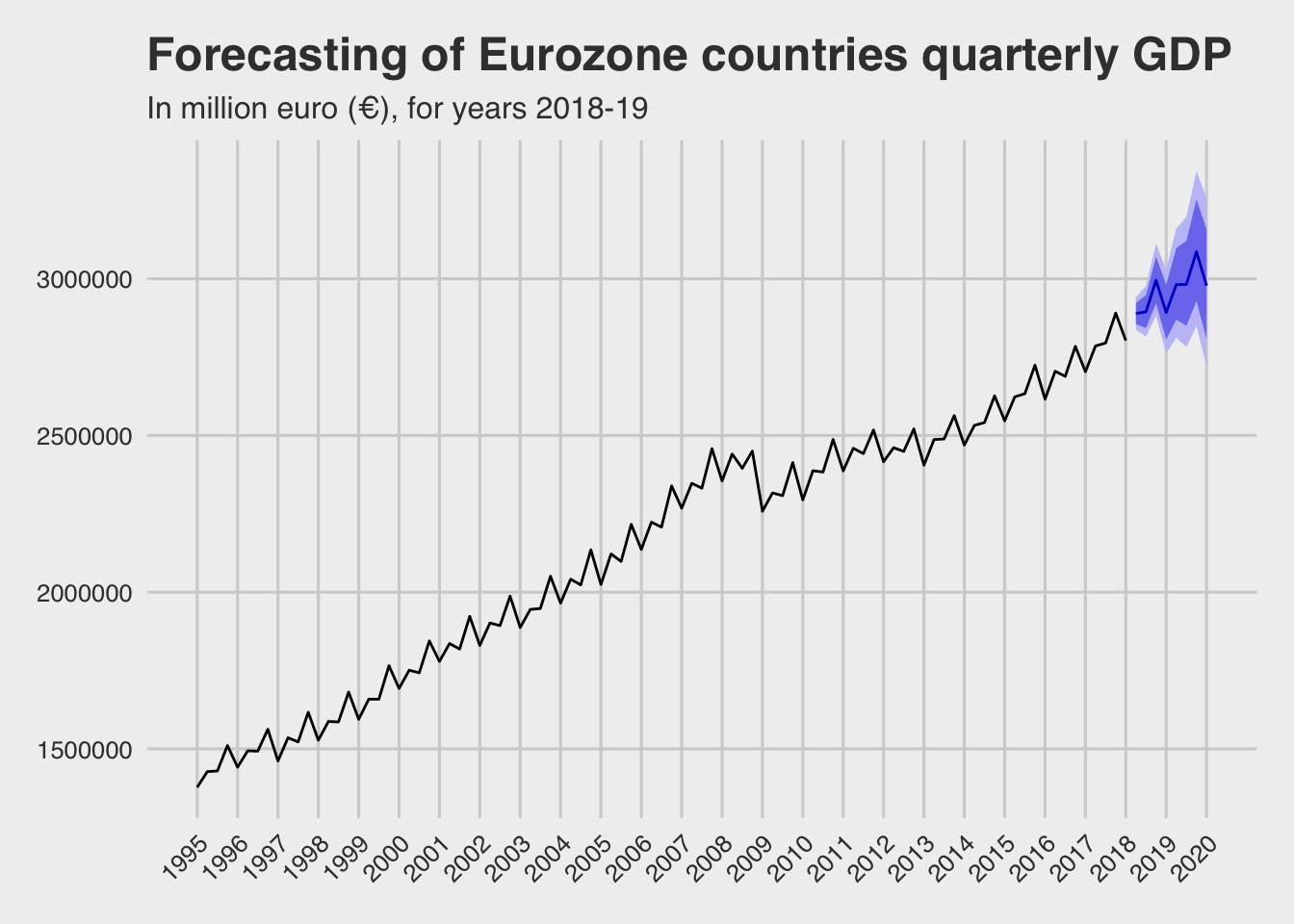
• It looks that GDP will keep growing in the next couple of years. In particular the forecasts for the future quarters are:

##         Point Forecast   Lo 80   Hi 80   Lo 95   Hi 95
## 2018 Q2        2888644 2854993 2922692 2837338 2940878
## 2018 Q3        2894625 2842396 2947813 2815131 2976364
## 2018 Q4        2995199 2921286 3070982 2882900 3111873
## 2019 Q1        2892031 2805760 2980954 2761138 3029128
## 2019 Q2        2981255 2869394 3097476 2811888 3160823
## 2019 Q3        2981904 2849446 3120520 2781726 3196488
## 2019 Q4        3086398 2928649 3252645 2848432 3344245

• It seems that by the end of 2019, there is a strong possibility that in one or more of the quarters of the year, the GDP will break the barrier of 3 trillion €

More models developed using other forecasting approaches, such as exponential smoothing(exponential smoothing methods with trend and seasonality Holt-Winters) & exponential triple smoothing, but the ARIMA model performance was better.

Full R code