Predict using classification methods
Feb 19, 2018 00:00 · 2760 words · 13 minute read
In this analysis i’ll try to build a model that will predict whether a tumor is malignant or benign, based on data from a study on breast cancer. Classification algorithms will be used in the modelling process.
The dataset
The data for this analysis refer to 569 patients from a study on breast cancer. The actual data can be found at UCI (Machine Learning Repository): https://archive.ics.uci.edu/ml/datasets/Breast+Cancer+Wisconsin+(Diagnostic). The variables were computed from a digitized image of a breast mass and describe characteristics of the cell nucleus present in the image. In particular the variables are the following
- radius (mean of distances from center to points on the perimeter)
- texture (standard deviation of gray-scale values)
- perimeter
- area
- smoothness (local variation in radius lengths)
- compactness (perimeter^2 / area - 1.0)
- concavity (severity of concave portions of the contour)
- concave points (number of concave portions of the contour)
- symmetry
- fractal dimension (“coastline approximation” - 1)
- type (tumor can be either malignant -M- or benign -B-)
# Load Libraries
library(dplyr)
library(tidyr)
# library(xda)
library(corrgram)
library(ggplot2)
library(ggthemes)
library(cluster)
library(caret)

# Insert dataset into R
med <- read.table("/Users/manos/Onedrive/Projects/R/Blogdown/data/cancer.txt", sep=",", header = TRUE)


# Discard the id column as it will not be used in any of the analysis below
med <- med[, 2:12]

# change the name of the first column to diagnosis
colnames(med)[1] <- "diagnosis"
Exploratory Analysis
It is essential to have an overview of the dataset. Below there is a box-plot of each predictor against the target variable (tumor). The log value of the predictors used instead of the actual values, for a better view of the plot.
# Create a long version of the dataset
med2 <- gather(med, "feature", "n", 2:11)

ggplot(med2)+
  geom_boxplot(aes(diagnosis, log(n)))+
  facet_wrap(~feature, scales = "free")+
  labs(title = "Box-plot of all predictors(log scaled) per tumor type",
       subtitle = "tumor can be either malignant -M- or benign -B-")+
 theme_fivethirtyeight()+
  theme(axis.title = element_text()) +
  ylab("Predictor's log value") +
  xlab('')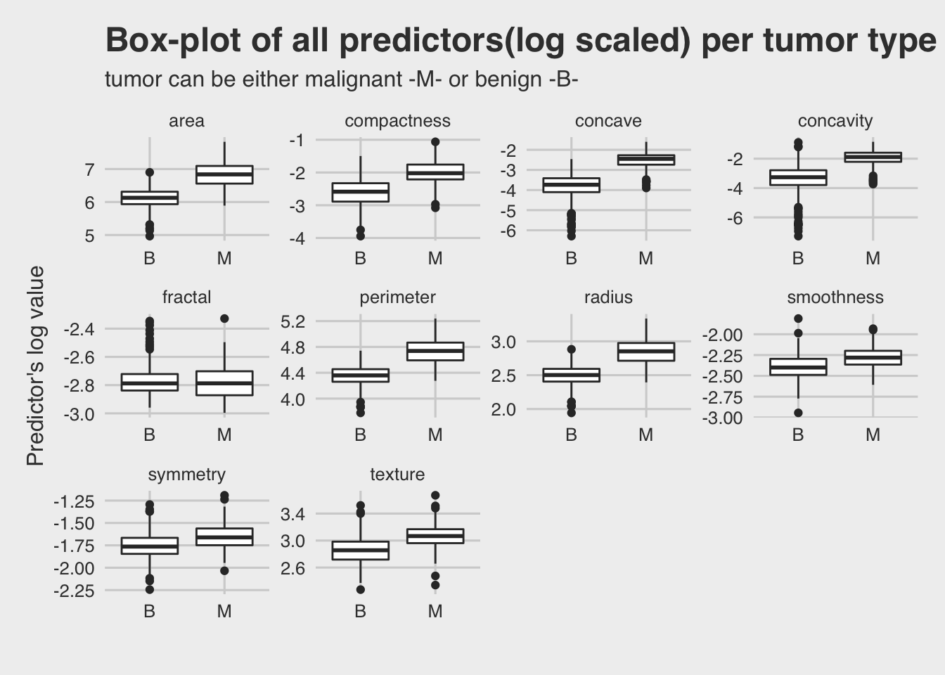
It seems that for most predictors the malignant level of tumor type has higher values than the benign level.
Now let’s see if the predictors are correlated. Below there is a scatter-plot matrix of all predictors.
# Scatterplot matrix of all numeric variables
pairs(~., data = med[, sapply(med, is.numeric)], main = "Scatterplot Matrix of variables")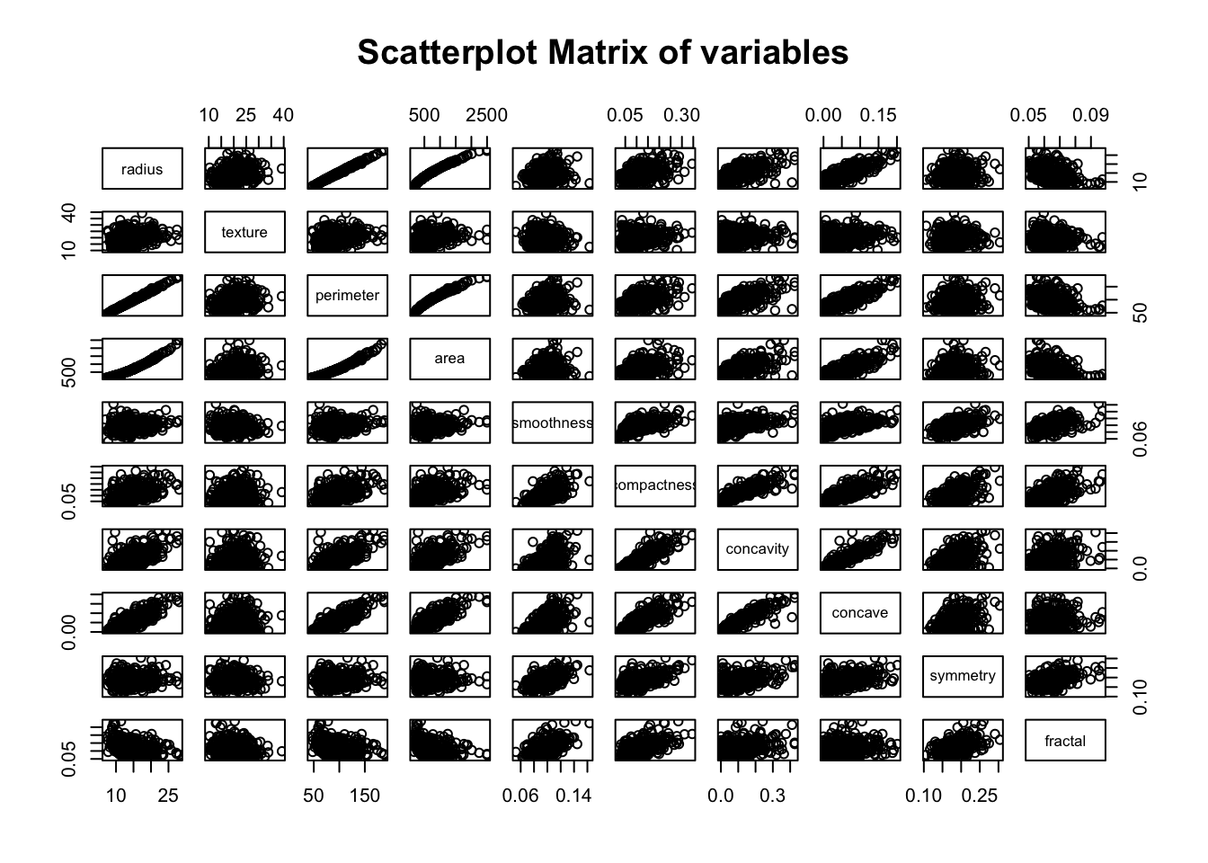
We can see that there are some predictors that are strongly related, as expected, such as radius, perimeter & area.
A correlogram will serve us better and quantify all correlations.
library(corrplot)

# Plot correlogram of numeric variables
corrplot(cor(med[,2:11]), type="lower", tl.srt = 90)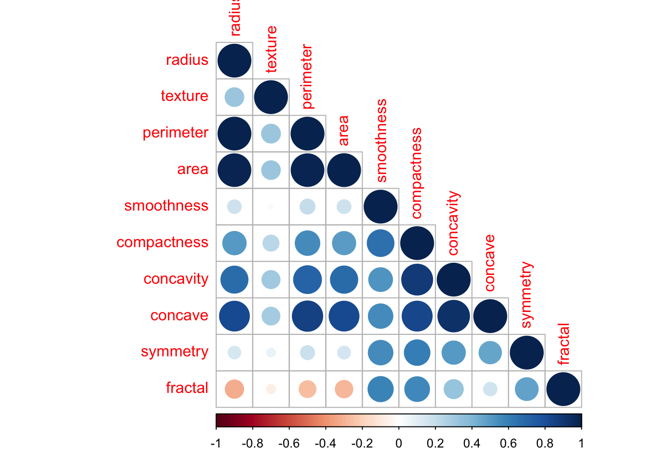
We can spot some less significant correlations, such as concave & concativity & compactness. Also concave against radius, perimeter & area.
Predicting using classification methods
In the first part of this analysis, the goal is to predict whether the tumor is malignant or benign based on the variables produced by the digitized image using classification methods. Classification is the problem of identifying to which of a set of categories (sub-populations) a new observation belongs, on the basis of a training set of data containing observations (or instances) whose category membership is known.
So we must develop a model that classifies (categorize) each tumor (case) to either malignant or benign.
Classification performed with 2 different methods, Logistic Regression and Decision Trees.
Feature selection
It is important to use only significant predictors while building the prediction model. You don’t need to use every feature at your disposal for creating an algorithm. You can assist the algorithm by feeding in only those features that are really important. Below there are some reasons for this:
- It enables the machine learning algorithm to train faster.
- It reduces the complexity of a model and makes it easier to interpret.
- It improves the accuracy of a model if the right subset is chosen.
- It reduces over-fitting.
In particular, i used the stepwise (forward & backward) logistic regression on the data, since the dataset is small. This method is computationally very expensive, so it is not recommended for very large datasets.
library(MASS)

med$diagnosis <- as.factor(med$diagnosis)

# Create a logistic regression model
glm <- glm(diagnosis ~ ., family=binomial(link='logit'), data = med)

# Run the stepwise regression
both <- stepAIC(glm, direction = "both")
## Start: AIC=168.13
## diagnosis ~ radius + texture + perimeter + area + smoothness +
## compactness + concavity + concave + symmetry + fractal
##
## Df Deviance AIC
## - compactness 1 146.14 166.14
## - perimeter 1 146.15 166.15
## - radius 1 146.44 166.44
## - fractal 1 146.78 166.78
## - concavity 1 147.23 167.23
## <none> 146.13 168.13
## - symmetry 1 148.44 168.44
## - area 1 151.63 171.63
## - concave 1 151.93 171.93
## - smoothness 1 152.42 172.42
## - texture 1 195.34 215.34
##
## Step: AIC=166.14
## diagnosis ~ radius + texture + perimeter + area + smoothness +
## concavity + concave + symmetry + fractal
##
## Df Deviance AIC
## - perimeter 1 146.22 164.22
## - radius 1 146.52 164.52
## - concavity 1 147.25 165.25
## - fractal 1 147.27 165.27
## <none> 146.14 166.14
## - symmetry 1 148.46 166.46
## + compactness 1 146.13 168.13
## - concave 1 151.93 169.93
## - area 1 152.00 170.00
## - smoothness 1 152.45 170.45
## - texture 1 195.48 213.48
##
## Step: AIC=164.22
## diagnosis ~ radius + texture + area + smoothness + concavity +
## concave + symmetry + fractal
##
## Df Deviance AIC
## - concavity 1 147.28 163.28
## <none> 146.22 164.22
## - fractal 1 148.30 164.30
## - symmetry 1 148.52 164.52
## + perimeter 1 146.14 166.14
## + compactness 1 146.15 166.15
## - radius 1 150.19 166.19
## - concave 1 152.19 168.19
## - area 1 153.35 169.35
## - smoothness 1 153.39 169.39
## - texture 1 195.93 211.93
##
## Step: AIC=163.28
## diagnosis ~ radius + texture + area + smoothness + concave +
## symmetry + fractal
##
## Df Deviance AIC
## - fractal 1 148.38 162.38
## <none> 147.28 163.28
## - symmetry 1 150.03 164.03
## + concavity 1 146.22 164.22
## + compactness 1 147.24 165.24
## + perimeter 1 147.25 165.25
## - radius 1 153.04 167.04
## - smoothness 1 153.61 167.61
## - area 1 156.64 170.64
## - concave 1 170.51 184.51
## - texture 1 197.40 211.40
##
## Step: AIC=162.39
## diagnosis ~ radius + texture + area + smoothness + concave +
## symmetry
##
## Df Deviance AIC
## <none> 148.38 162.38
## - symmetry 1 150.68 162.68
## + fractal 1 147.28 163.28
## + compactness 1 147.45 163.45
## + perimeter 1 147.74 163.74
## + concavity 1 148.30 164.30
## - radius 1 153.44 165.44
## - smoothness 1 154.44 166.44
## - area 1 157.38 169.38
## - concave 1 172.31 184.31
## - texture 1 198.83 210.83# Print the summary of the stepwise model
summary(both)##
## Call:
## glm(formula = diagnosis ~ radius + texture + area + smoothness +
## concave + symmetry, family = binomial(link = "logit"), data = med)
##
## Deviance Residuals:
## Min 1Q Median 3Q Max
## -1.94562 -0.15248 -0.04346 0.00366 2.89274
##
## Coefficients:
## Estimate Std. Error z value Pr(>|z|)
## (Intercept) -8.61085 8.33550 -1.033 0.30159
## radius -2.72515 1.17554 -2.318 0.02044 *
## texture 0.38522 0.06430 5.991 2.09e-09 ***
## area 0.04308 0.01428 3.017 0.00255 **
## smoothness 58.37855 23.49622 2.485 0.01297 *
## concave 73.70154 16.21489 4.545 5.49e-06 ***
## symmetry 15.56212 10.25705 1.517 0.12921
## ---
## Signif. codes: 0 '***' 0.001 '**' 0.01 '*' 0.05 '.' 0.1 ' ' 1
##
## (Dispersion parameter for binomial family taken to be 1)
##
## Null deviance: 751.44 on 568 degrees of freedom
## Residual deviance: 148.39 on 562 degrees of freedom
## AIC: 162.39
##
## Number of Fisher Scoring iterations: 9# Select only important variables
med <- med[, c("diagnosis","radius", "texture", "area", "smoothness", "concave", "symmetry")]After reviewing the stepwise selection, it was decided the following predictors to be used for all model building:
- radius (mean of distances from center to points on the perimeter)
- texture (standard deviation of gray-scale values)
- area
- smoothness (local variation in radius lengths)
- concave points (number of concave portions of the contour)
- symmetry
Logistic Regression
Logistic regression is a parametric statistical learning method, used for classification especially when the outcome is binary. Logistic regression models the probability that a new observation belongs to a particular category. To fit the model, a method called maximum likelihood is used. Below there is an implementation of logistic regression.
# Create a vector with the 70% of the dataset with respect to diagnosis variable
set.seed(1)
inTrain = createDataPartition(med$diagnosis, p = .7)[[1]]


# Assign the 70% of observations to training data
training <- med[inTrain,]

# Assign the remaining 30 % of observations to testing data
testing <- med[-inTrain,]
# Build the model
glm_model <- glm(diagnosis~., data = training, family = binomial)## Warning: glm.fit: fitted probabilities numerically 0 or 1 occurredsummary (glm_model)##
## Call:
## glm(formula = diagnosis ~ ., family = binomial, data = training)
##
## Deviance Residuals:
## Min 1Q Median 3Q Max
## -1.92738 -0.09810 -0.01796 0.00039 2.74892
##
## Coefficients:
## Estimate Std. Error z value Pr(>|z|)
## (Intercept) -7.41467 11.66161 -0.636 0.524895
## radius -4.32564 1.72858 -2.502 0.012334 *
## texture 0.46873 0.09673 4.846 1.26e-06 ***
## area 0.06636 0.02171 3.057 0.002234 **
## smoothness 81.42115 32.27956 2.522 0.011657 *
## concave 75.92517 22.81446 3.328 0.000875 ***
## symmetry 31.63111 14.47792 2.185 0.028905 *
## ---
## Signif. codes: 0 '***' 0.001 '**' 0.01 '*' 0.05 '.' 0.1 ' ' 1
##
## (Dispersion parameter for binomial family taken to be 1)
##
## Null deviance: 527.285 on 398 degrees of freedom
## Residual deviance: 89.276 on 392 degrees of freedom
## AIC: 103.28
##
## Number of Fisher Scoring iterations: 9By looking at the summary output of the logistic regression model we can see that almost all coefficients are positive, indicating that higher measures mean higher probability of a malignant tumor.
An important step here is to evaluate the predicting ability of the model. Because the model’s predictions are probabilities, we must decide the threshold that will split the two possible outcomes. At first i’ll try the default threshold of 0.5. Below there is a confusion matrix of with predictions using this threshold.
options(scipen=999)

# Apply the prediction
prediction <- predict(glm_model, newdata= testing, type = "response")
prediction <- ifelse(prediction > 0.5, "M", "B")

# Check the accuracy of the  prediction model by printing the confusion matrix.
print(confusionMatrix(as.factor(prediction), testing$diagnosis), digits=4)
## Confusion Matrix and Statistics
##
## Reference
## Prediction B M
## B 102 7
## M 5 56
##
## Accuracy : 0.9294
## 95% CI : (0.8799, 0.963)
## No Information Rate : 0.6294
## P-Value [Acc > NIR] : <0.0000000000000002
##
## Kappa : 0.8477
##
## Mcnemar's Test P-Value : 0.7728
##
## Sensitivity : 0.9533
## Specificity : 0.8889
## Pos Pred Value : 0.9358
## Neg Pred Value : 0.9180
## Prevalence : 0.6294
## Detection Rate : 0.6000
## Detection Prevalence : 0.6412
## Balanced Accuracy : 0.9211
##
## 'Positive' Class : B
## The overall accuracy of the model is 96.47 % (3.53 % error rate). But in this specific case we must distinguish the different types of error. In other words there are two types of error rate, type I & type II errors. In our case these are similar (type II error = 3.74% & type I error = 3.17%). Type I error means that a benign tumor is predicted to be malignant & type II error when a malignant tumor is predicted to be benign. Type II error is more expensive and we must find ways to eliminate it(even if it increases type I error).
Below i increased the threshold to 0.8, which changed the prediction model.
options(scipen=999)


# Apply the prediction
prediction <- predict(glm_model, newdata= testing, type = "response")
prediction <- ifelse(prediction > 0.8, "M", "B")

# Check the accuracy of the  prediction model by printing the confusion matrix.
print(confusionMatrix(as.factor(prediction), testing$diagnosis), digits=4)
## Confusion Matrix and Statistics
##
## Reference
## Prediction B M
## B 106 7
## M 1 56
##
## Accuracy : 0.9529
## 95% CI : (0.9094, 0.9795)
## No Information Rate : 0.6294
## P-Value [Acc > NIR] : <0.0000000000000002
##
## Kappa : 0.8971
##
## Mcnemar's Test P-Value : 0.0771
##
## Sensitivity : 0.9907
## Specificity : 0.8889
## Pos Pred Value : 0.9381
## Neg Pred Value : 0.9825
## Prevalence : 0.6294
## Detection Rate : 0.6235
## Detection Prevalence : 0.6647
## Balanced Accuracy : 0.9398
##
## 'Positive' Class : B
## Although the overall accuracy of the model remains the same, now the type II error is eliminated but the type I error is increased. In other words, we now have a model that predicts perfectly a malign tumor but it also wrongly predicts some benign tumors as malignant (9.5%).
Decision Trees
Decision trees consist of a series of split points, often referred to as nodes. In order to make a prediction using a decision tree, we start at the top of the tree at a single node known as the root node. The root node is a decision or split point, because it places a condition in terms of the value of one of the input features, and based on this decision we know whether to continue on with the left part of the tree or with the right part of the tree. We repeat this process of choosing to go left or right at each inner node that we encounter until we reach one of the leaf nodes. These are the nodes at the base of the tree, which give us a specific value of the output to use as our prediction.
# Create a vector with the 70% of the dataset with respect to diagnosis variable
set.seed(1)
inTrain = createDataPartition(med$diagnosis, p = .7)[[1]]


# Assign the 70% of observations to training data
training <- med[inTrain,]

# Assign the remaining 30 % of observations to testing data
testing <- med[-inTrain,]

# Set seed (in order all results to be fully reproducible) and apply a prediction
#Model with all variables
set.seed(2)
model.all <- train(diagnosis ~ ., method="rpart", data = training)

# Apply the prediction
prediction <- predict(model.all, newdata= testing)

# Check the accuracy of the  prediction model by printing the confusion matrix.
print(confusionMatrix(prediction, testing$diagnosis), digits=4)
## Confusion Matrix and Statistics
##
## Reference
## Prediction B M
## B 95 4
## M 12 59
##
## Accuracy : 0.9059
## 95% CI : (0.8517, 0.9452)
## No Information Rate : 0.6294
## P-Value [Acc > NIR] : < 0.0000000000000002
##
## Kappa : 0.8034
##
## Mcnemar's Test P-Value : 0.08012
##
## Sensitivity : 0.8879
## Specificity : 0.9365
## Pos Pred Value : 0.9596
## Neg Pred Value : 0.8310
## Prevalence : 0.6294
## Detection Rate : 0.5588
## Detection Prevalence : 0.5824
## Balanced Accuracy : 0.9122
##
## 'Positive' Class : B
## When performing the Decision Trees, as seen from the output, the overall prediction rate is 94.1% (5.9% error rate), which for the specific domain, is relatively low. In particular, the type II error is 5.61% & type I error = 6.35%. The model’s predictive performance is poorer than the previous one (logistic regression).
Now let’s create a classification tree plot of the model.
library(rpart.plot)

# Plot the Classification Tree
rpart.plot(model.all$finalModel, main = "Classification Tree of tumor type prediction")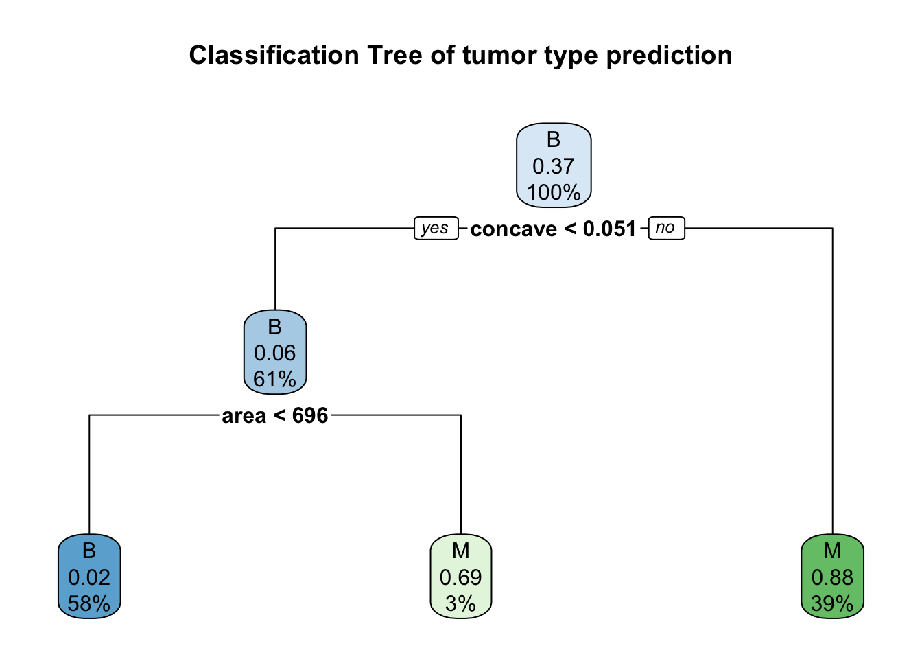
From the plot above, we can assume that concave and texture are the most import important predictors for tumor type (splits on the classification trees).
Results
Finally, after building various models using different algorithms, the logistic regression model is chosen based on it’s performance (details on the table below).
| Prediction model | Overall Error rate | Type I error | Type II error |
|---|---|---|---|
| Logistic regression | 3.5 % | 9.5 % | 0 % |
| Decision Trees | 5.9 % | 5.6 % | 6.35 % |
In particular, especially after adjusting the threshold, it eliminated the type II error (wrongly predict malignant tumors as benign). This is really important in this specific problem.
As expected parametric methods, such as logistic regression, are performing better in this case, where we have a small dataset (569 observations).
While our analysis is an interesting step it is based on a limited sample of cases. A larger sample of cases, would probably lead us to a better classification model.